The Magrathea Manual: Coordinated Agent Modelling By Example
Contents
- 1 The Magrathea Manual Contents
- 2 Examples
- 2.1 Example 1. Point coordinator representing an interaction
- 2.2 Example 2. Point coordinator representing a complex
- 2.3 Example 3. Point coordinator representing a compartment.
- 2.4 Example 4. Plane coordinator representing a membrane section.
- 2.5 Example 5. Line coordinator representing a microtubule.
- 2.6 Example 6. Coordinators and rules.
The Magrathea Manual Contents
The Magrathea Manual: Coordinated Agent Modelling Explained
The Magrathea Manual: Coordinated Agent Modelling By Example
The Magrathea Manual: Building Coordinated Agent Models
Magrathea Installation and Use
Example model files for Magrathea
Examples
In this section, we describe a number of examples that demonstrate the capabilities of the prototype implementation of the CAM method.
Examples are described using movies and explanatory text that notes how molecules and coordinators are defined to achieve the described model capabilities. Model files are available for each example that detail the exact implementation of these methods. These model files are available at Example model files for Magrathea. These files may be directly copied and pasted into a file called “model.txt” that exists in the same directory as the magrathea.tz prototype script.
The user is referred to the Magrathea Manual: Building Coordinated Agent Models for a more detailed description of the syntax used in these model files. These model files are working examples; see the sections on Installation and Use for details.
Example 1. Point coordinator representing an interaction
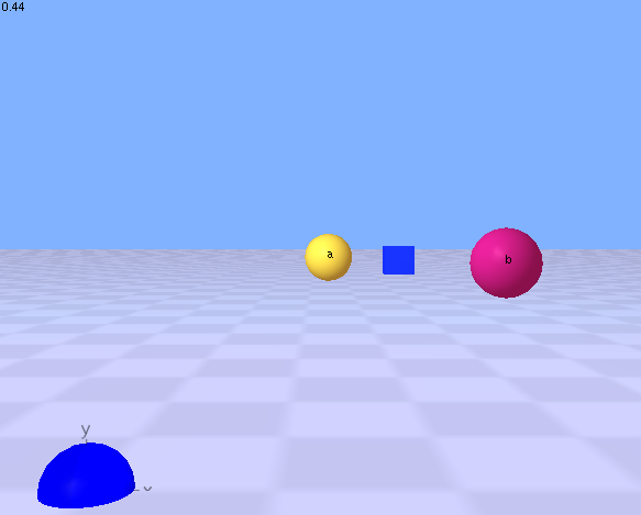  |
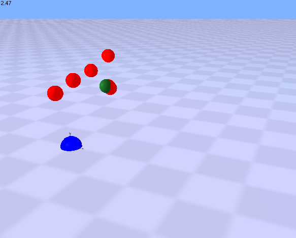
This is a simple example using two molecules labeled a and b. Each molecule is represented by a sphere with a radius of 1 unit and each has dynamic neighborhood sizing turned on. At each time step, the two molecules increase their neighborhood size by 1 until each is found within the other’s neighborhood. At this point, a coordinator (represented by a cube) is created and moved to a position midway between the two molecules. At each time-step thereafter, the coordinator moves the two molecules into position on an imaginary sphere drawn around the coordinator and holds them in this position using a spring function.
Click on the picture to view the movie. Your web browser requires a plugin (like Quicktime) that is capable of viewing mpeg files. Click the back button in your browser to return here when you are done viewing the movie. See interaction1.txt model file at Example model files for Magrathea The blue sphere at the centre of this image is a marker used in all simulations to show the world centre with x and y axes marked. A floor is also shown in all simulations for the z=0 plane. If dynamic neighborhood sizing is turned off (set to 0), the two molecules will most likely not collide with one another and will continue in a random walk through the simulation. |
Example 2. Point coordinator representing a complex
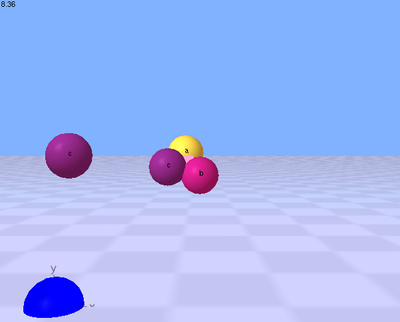  |
This is a simple example using three molecule types labeled a, b and c. There are two molecules of type c. Each molecule is represented by a sphere with a radius of 1 unit and each has dynamic neighborhood sizing turned on. At each time step, the molecules increase their neighborhood size by 1 until at least two find one another within the other’s neighborhood. At this point, a coordinator (represented by a cube) is created and moved to a position midway between the molecules. This coordinator represents a complex with stochiometry 1a, 1b, and 1c. Only 2 molecules (of the 4 present) are required to initiate the formation of the complex since the assembly has no specified order. The third may join this coordinator later.
At each time-step thereafter, the coordinator moves all three molecules into position on an imaginary sphere drawn around the coordinator and holds them in this position using a spring function. The fourth (extra) molecule c remains unassembled. Click on the picture to view the movie. Your web browser requires a plugin (like Quicktime) that is capable of viewing mpeg files. Click the back button in your browser to return here when you are done viewing the movie. See complex1.txt model file at Example model files for Magrathea
|
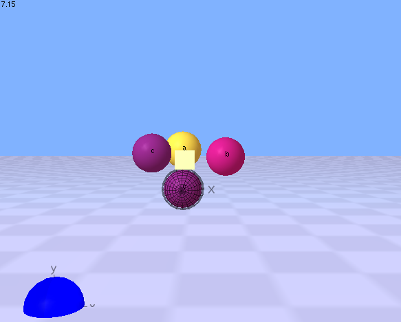  |
A second model file (complex2.txt) specifies a coordinator with a stoichiometry of 1a, 1b, 2c so all four molecules are included in the final complex.
Click on the picture to view the movie. Your web browser requires a plugin (like Quicktime) that is capable of viewing mpeg files. Click the back button in your browser to return here when you are done viewing the movie. See complex2.txt model file at Example model files for Magrathea You may notice at the beginning of the complex2.mpeg movie that a coordinator first forms between the 2 c subunits and then this coordinator moves between all four subunits. The coordinator first forms between the two c subunits since they are closest to one another in the simulation. When subunits a and b detect either of these c subunits in their neighborhood, they first check for existing coordinators that they can join. When a and b join this existing coordinator, the coordinator moves to a position midway between all four subunits. |
Example 3. Point coordinator representing a compartment.
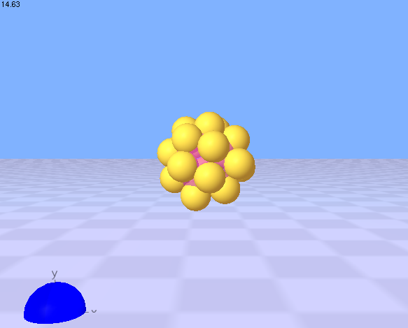  |
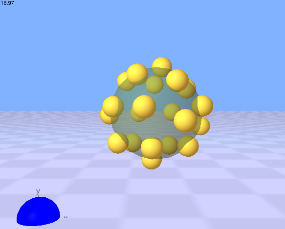
This is a simple example of a coordinator used to represent a compartment.
Twenty instances of a single molecule type become members of this coordinator (i.e. they define its boundary). The 20 molecules are constrained to movement on the surface of an imaginary sphere whose surface area is equivalent to the sum of the cross-sectional areas of the 20 molecules. The coordinator representing a compartment must be a point coordinator (see geometricType). In this simulation it is represented by a translucent sphere that grows from an initial size to the size of the imaginary sphere as molecules are added to it. This size increase is dependent on the line isSizeDynamic 1 The sphere is used to handle collisions with other molecules that are not a part of the compartment coordinator (see below). Click on the above image to view the movie of the simulation. See compartment.1.txt model file at Example model files for Magrathea
|
  |
Molecules may also be described that have a larger effective radius than what is rendered. This allows for the compartment to be delimited by “marker molecules” without having to cover the entire surface of the compartment. An example is shown in compartment.2.txt model file. A single change was made to the above model file to achieve this. See the line
shape Sphere 1 2 Click on the above image to view the movie of the simulation. See See compartment.2.txt model file at Example model files for Magrathea |
Example 4. Plane coordinator representing a membrane section.
  |
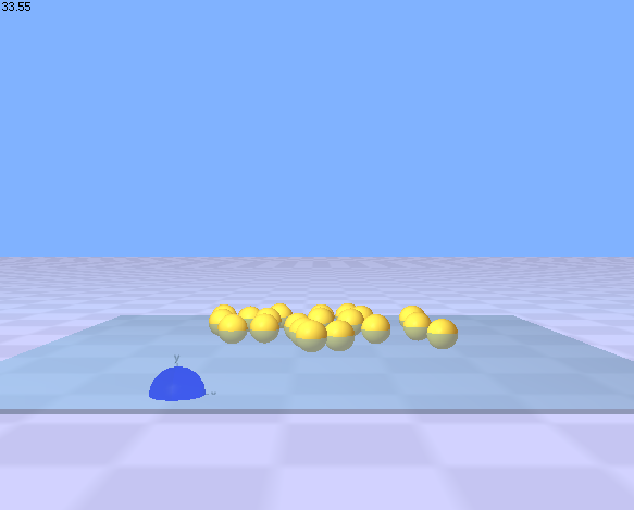
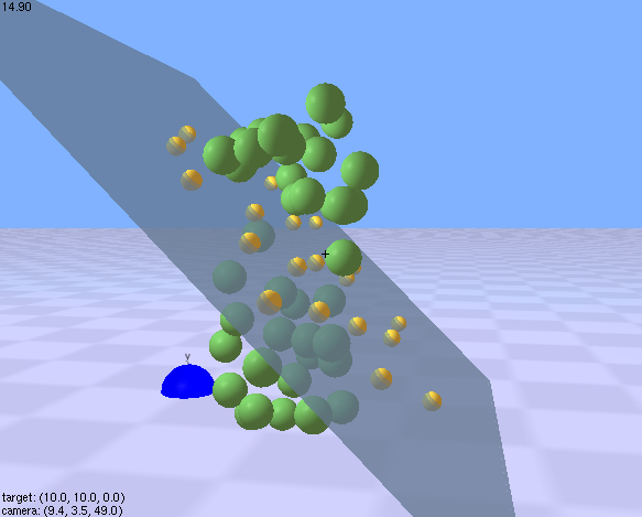
This is a simple example in which 20 instances of one molecule type are all potential members of a plane coordinator. The molecules are moved to the surface of the plane where they can move randomly in that surface but they cannot move out of the surface.
Plane coordinators are generally created at the beginning of the simulation and will persist for the duration of the simulation (i.e. they are not dynamically created according to context ant they cannot be destroyed). Further, plane coordinators can be specified as non-mobile so the plane remains stationary during the simulation (otherwise, the plane would move to maintain a centre that is midway between the positions of the member molecules). Lastly, like point coordinators representing compartments, the plane coordinator can increase in size from its starting size as member molecules join. These coordinator characteristics are encoded by the lines isCreationDynamic 0 isMobile 0 isSizeDynamic 1 in the [coordinatorType] section of the model file. Click on either image to view the movie of the simulation. Both figures link to the same movie. See See membrane.1.txt model file at Example model files for Magrathea Finally, the orientation of the plane at the start of the simulation can be changed using the orientation line. This model file can be altered by uncommenting (removing the # symbol) in front of one of the lines beginning with #orientation to see this effect. An example is shown in the bottom figure. Both figures link to the same movie. |
|
| |
  |
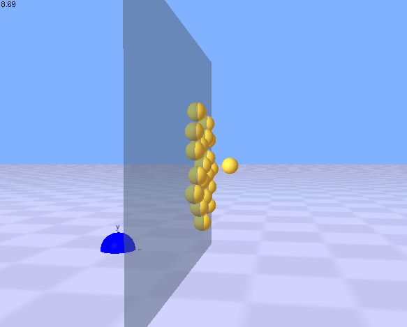
This example adds non-membrane molecules to either side of the membrane to show that collisions are handled with the surface of the membrane.
Click on either image to view the movie of the simulation. Both figures link to the same movie. See See membrane.2.txt model file at Example model files for Magrathea Again, the orientation of the plane at the start of the simulation can be changed using the orientation line. This model file can be altered by uncommenting (removing the # symbol) in front of one or more of the lines beginning with #orientation to see this effect. An example is shown in the bottom figure. |
Example 5. Line coordinator representing a microtubule.
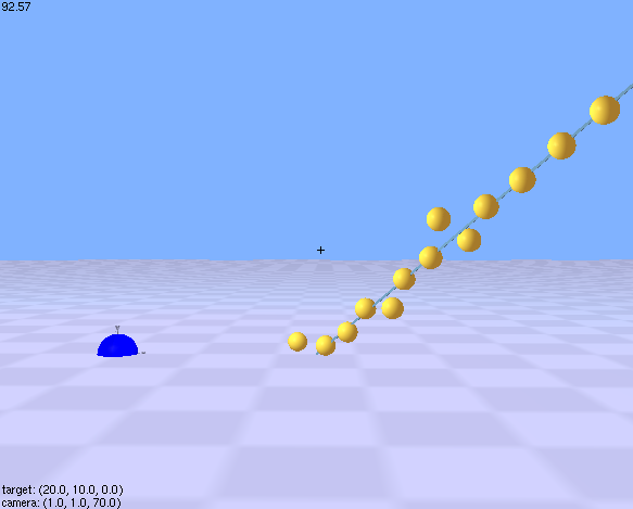  |
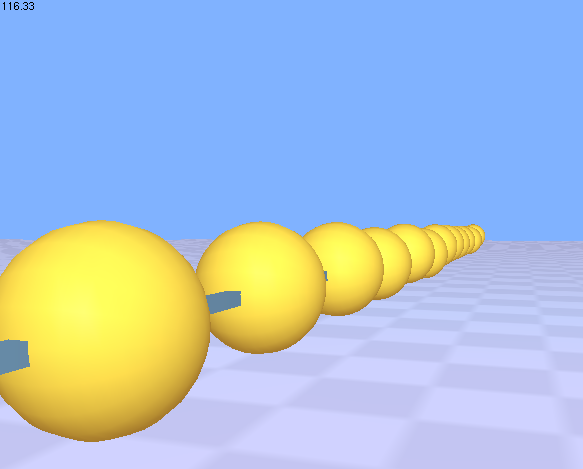
This is a simple example in which 20 instances of one molecule type are all potential members of a line coordinator. The molecules are moved to the line where they can move randomly along that line.
Like the plane coordinator described in the example above, the line coordinator shown in this model is created at the beginning of the solution and persists throughout the simulation without changing position. Click on either image to view the movie of the simulation. Both figures link to the same movie. The figures show the line coordinator in two different starting orientations. See See microtubule.1.txt model file at Example model files for Magrathea The associated movie in the example directory demonstrates use of camera movements during the simulation. The model file also shows an example of populating a simulation with a set of molecules that are arranged in a line using the instantiate line in the model file: instantiate 20 random cylindrical volume 10 15 10 0 1 0 0 35 See the section on building model files for more details. |
Example 6. Coordinators and rules.
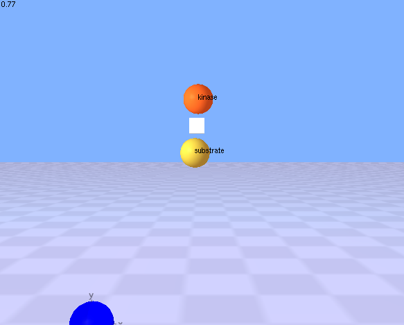  |
This is a simple demonstration of the use of rules by coordinators.
This example shows a substrate (molecule 1) that undergoes a state-change (phosphorylation) upon interaction with a kinase (molecule 2). The state change is visualized by a colour change. A single coordinator type uses three rules to control 1) the assembly of unphosphorylated substrate with the kinase, 2) the phosphorylation (state change) of the substrate and 3) the disassembly of the kinase-substrate complex after phosphorylation. After the substrate is phosphorylated, it can no longer be considered as a potential member of this coordinator and so the two molecules drift apart.
|
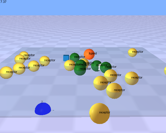  |
This demonstration shows a somewhat more complex use of rules to demonstrate the process of lateral signalling.
In this example, a ligand molecule binds to a membrane-bound receptor. On binding, the receptor changes state (becomes activated) as indicated by a colour change. The receptor in this new state also gains the ability to bind to and activate other membrane bound receptors. The overall effect is that a single ligand-receptor binding event initiates a lateral cascade of receptor activation events. Click on the picture to view the movie. Your web browser requires a plugin (like Quicktime) that is capable of viewing mpeg files. Click the back button in your browser to return here when you are done viewing the movie. See rules.2.txt model file at Example model files for Magrathea |
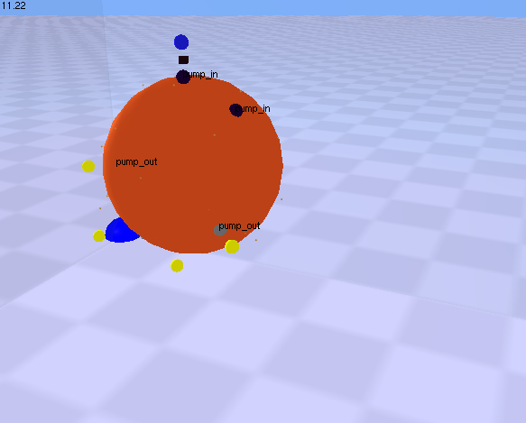  |
This demonstration shows a set of rules that control translocation into and out of a spherical compartment. A number of ligand molecules (blue) bind to a surface receptor (black) on the orange compartment’s surface. The coordinator handling this ligand receptor interaction encodes a rule that translocates the ligand into the orange compartment and changes the state of the ligand such that it is capable of binding to a second receptor (grey) that is also a surface component of the orange compartment. This state change is associated with a colour change for the ligand molecule (blue to yellow). A second coordinator handles the interaction between the ligand and the second receptor and encodes a rule that translocates the ligand out of the orange compartment. Once the ligand is outside the compartment, its state (yellow) prevents it from assembling with the importing receptor (black) for a second time.
Click on the picture to view the movie. Your web browser requires a plugin (like Quicktime) that is capable of viewing mpeg files. Click the back button in your browser to return here when you are done viewing the movie. See rules.3.txt model file at Example model files for Magrathea |
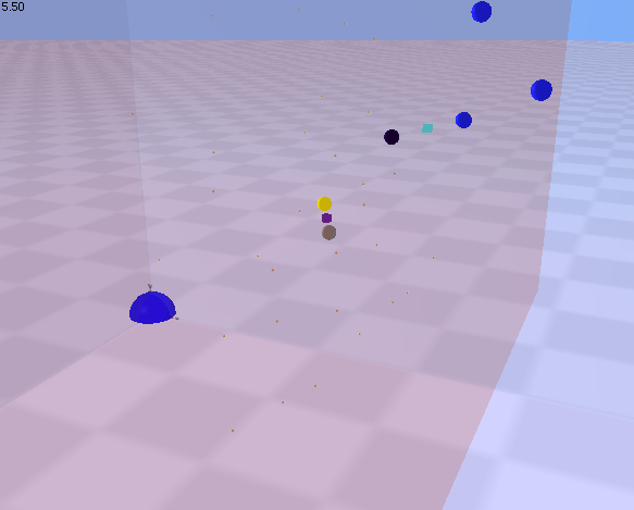  |
This example shows a screen shot of a simulation similar to the last except that it uses a planar coordinator representing a membrane section (instead of a compartment).
Planar coordinators are not compartments in the sense that molecules can move into and out of them. Instead, they represent barriers within a compartment (in this case the simulation) that molecules can move past with the help of a mediator molecule (the black and grey receptors). Click on the picture to view the movie. Your web browser requires a plugin (like Quicktime) that is capable of viewing mpeg files. Click the back button in your browser to return here when you are done viewing the movie. See rules.4.txt model file at Example model files for Magrathea |
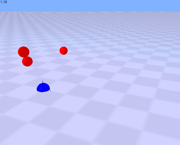  |
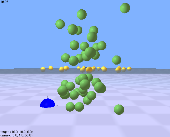
Rules may also be specified for molecules. These rules are essential for describing “spontaneous” events that occur for a single molecule regardless of its context (membership with a coordinator). For example, a molecule may spontaneously undergo some feature-state (even in the absence of any other interacting molecules). Similarly, the molecule may be spontaneously destroyed. These types of molecule events are may be dependent on a specific feature-state of the molecule and may also be associated with a probability for the event at each time-step of the simulation. These rules may also be used to represent molecules that are at the “edge” of a model; processes leading to the destruction and creation of these molecules are not described in the model but are instead modeled as a molecule-associated rule.
Click on the picture to view the movie. Your web browser requires a plugin (like Quicktime) that is capable of viewing mpeg files. Click the back button in your browser to return here when you are done viewing the movie. See rules.5.txt model file at Example model files for Magrathea |
  |
This movie shows a slightly more complicated example that employs feature-state changes prior to creating or destroying a molecule instance.
Click on the picture to view the movie. Your web browser requires a plugin (like Quicktime) that is capable of viewing mpeg files. Click the back button in your browser to return here when you are done viewing the movie. See rules.6.txt model file at Example model files for Magrathea |